By Patrick Valentine, PhD, Brittany Malin and April Labonte
Uyemura International Corporation
Southington CT
Abstract
Design of Experiments (DoE) drives effective product and process design, development, and improvement. While DoE principles are proven, manufacturing environments often suffer from limited access to equipment and resources. Field constraints complicate the selection, execution, and analysis of experiments. This paper demonstrates how to apply core DoE principles despite real-world challenges, providing a practical reference guide and a detailed example.
Keywords: Design of experiments, field constraints, DoE design reference guide, training
Introduction
Design of experiments (DoE) is an efficient method for planning experiments. DoE involves intentionally changing one or more input-process factors—also known as independent variables—to observe how these changes affect output or response variables (the outcomes measured in an experiment). DoE is often used for product and process design, development, and improvement. To maximize information and minimize time, resources, or cost, a properly chosen experimental design is needed.
An experimental design is the creation of a detailed experimental plan that is completed before experimenting. A good experimental design incorporates process knowledge, sound statistical procedures, and experience. Process knowledge includes technical knowledge and intellectual capacity gained from previous projects or problems. Statistical procedures include a basic understanding of ANOVA (analysis of variance) tables and how to interpret residual plots. While experience takes time, developing a sound experimental design is needed to ensure efficient time utilization and valid, relevant results.
Properly defining the response variable is key to ensuring the experiment’s validity. The engineer must decide what will be measured, how it will be expressed, and whether the response is continuous (can take any value within a range, like weight or temperature) or categorical (fits into groups, like pass/fail). In general, continuous responses are preferred due to greater analytical sensitivity [1]. Clear operational definitions reduce ambiguity and support consistent data collection. Reliable measurement systems and stable process conditions are also needed. These ensure that statistical significance reflects true process behavior and not measurement variation [2].
Design of experiments is often organized into six steps: define the objective, design the experiment, execute the study, analyze the data, conduct confirmation runs, and report conclusions [3]. The design phase includes selecting responses, defining factor ranges, and choosing an experimental design. Data analysis often uses ANOVA and regression modeling to assess model adequacy and estimate effects. Certain requirements must be met to ensure correct, unambiguous, and defensible conclusions from DoEs. These requirements include an equitable sample, process stability, statistical and practical significance, and truth [2]. Confirmation runs validate predictions and increase confidence in conclusions.
Field Constraints
Although DoE principles are well established, their practical application is often influenced by environmental and operational realities. Traditional discussions of DoE often assume ideal experimental conditions. In practice, experiments are frequently conducted under field constraints. These constraints influence factor selection, run order, and replication strategy, often requiring a compromise between theoretical optimality and practical feasibility [4]. While the statistical principles of DoE remain unchanged, their implementation must often be adapted to field constraints.
In a production environment, production demands take priority over DoEs. This can affect sample size (the number of individual units tested), replication (repeating tests to confirm results), and randomization (assigning conditions or samples in a random order), because time and access to equipment can be limited. Once access is granted, performing DoEs on a production line introduces added challenges. There are uncontrollable factors, such as noise (random variation from environmental sources), and some factors may be hard to change. Safety is also a concern when working with automated equipment. Additionally, test vehicles (materials or assemblies used for testing) used for experimentation are often not truly representative of actual products. Producing this material may be costly and time-consuming. Test coupons (small samples designed to mimic product sections) are commonly substituted, but they may not fully replicate the real work being produced.
Design of Experiment for Field Constraints
Once practical limitations are understood, the next step is selecting an experimental design that can generate meaningful information within those constraints. Several experimental designs are commonly used in production environments. These designs vary in complexity (the number of factors and interactions considered), statistical power (the ability to detect a real effect), and the number of experimental runs required. Each design offers specific advantages depending on the number of factors being studied and the available experimental flexibility. The following sections summarize several commonly used experimental designs and their key characteristics. A DoE design reference guide is shown in Table 1.
One-Factor-at-a-Time (OFAT) Designs
One-factor-at-a-time experimentation changes one experimental factor—such as temperature, concentration, or pressure—while all other variables are held constant. This approach is easy to implement and needs little statistical planning. This simplicity helps explain its widespread use in industrial settings. OFAT is helpful when factors are very difficult to change or when flexibility is limited. For example, adjusting copper concentration in an electroplating via-fill tank may require substantial preparation, so it may be changed only once per experiment. However, OFAT cannot usually estimate interactions (how two or more factors might work together to affect an outcome) and gives limited insight into complex processes. As a result, it is generally not recommended when multiple factors may influence the response.
One-Way ANOVA Designs
One-way analysis of variance designs evaluate the effect of a single factor with two or more levels on a response variable. These designs extend the two-sample t-test, which compares means between two groups, to cases with multiple group means. At least two observations per factor level are required, and equal sample sizes are generally preferred. When sample sizes are unequal or group variances differ, Welch’s ANOVA provides a more robust alternative because it does not assume equal population variances. One-way ANOVA designs are useful when the objective is to compare treatments or process conditions with a single factor.
22 Full Factorial Designs
A 22 full factorial design studies two factors at two levels each. This requires four runs and allows estimation of both main effects and their interaction. All combinations of factor levels are tested, so factorial designs provide more information than OFAT with the same factors. Center points (an additional setting for each factor at a value midway between its two levels) can be added to detect curvature in responses. Statistical models derived from factorial experiments generally follow a hierarchical structure, meaning that interaction terms are included only when their corresponding main effects are also present. The 2² factorial design efficiently studies two factors with four runs.
23 Full Factorial Designs
A 23 full factorial design extends the approach to three factors, each at two levels. This needs eight runs and allows estimation of three main effects, three two-factor interactions, and one three-factor interaction. As with smaller factorial designs, center points may be added to check for curvature in the response surface. Studying several factors simultaneously allows engineers to spot potential interactions that might not surface during OFAT. However, the number of runs rises quickly as more factors are added. Careful planning is needed when choosing factorial designs with many factors.
D-Optimal Designs
D-optimal designs belong to a broader class of experimental designs known as alphabet-optimal designs. These designs are generated algorithmically to optimize a specific statistical criterion associated with the model's information matrix. D-optimal is one of the most commonly used designs. Optimal designs are particularly useful when experimental regions contain constraints or when the number of possible runs must be minimized. Unlike classical factorial designs, optimal designs are not inherently orthogonal and are typically constructed for a specific statistical model. Despite this limitation, optimal designs provide a flexible approach when traditional designs are not feasible.
Taguchi L9 Designs
Taguchi designs are orthogonal arrays that allow multiple factors to be evaluated using a relatively small number of experimental runs. The L9 array is commonly used for experiments involving four factors at three levels each, although mixed-level factors may also be incorporated. Taguchi methods emphasize robust parameter design and use signal-to-noise ratios to evaluate performance. These designs are efficient for screening factors and identifying influential variables. However, the alias structure of Taguchi arrays can be complex, leading to confounding among certain effects. Careful interpretation of results is therefore required.
Plackett–Burman Designs
Plackett–Burman designs are screening designs used to evaluate a large number of factors with relatively few experimental runs. These designs estimate main effects but do not provide reliable estimates of interaction effects. For example, a 12-run Plackett–Burman design can evaluate up to eleven factors simultaneously. One advantage of this design is that the correlations among factors are weak, distributing potential interaction effects across the design matrix. Plackett–Burman designs are commonly used during early troubleshooting to identify which factors may influence the response. Once important factors are identified, more detailed experimental designs can be used to investigate interactions and optimize the system.
Table 1. DoE design reference guide.| Design of Experiment | Maximum Factors (n) | Factor Levels | Runs | Interactions | Hard to Change Factor |
| OFAT | 5 | 2 | n +1 | No | Yes |
| One-Way ANOVA | 1 | 6 | * | N/A | Yes |
| 22 Full Factorial | 2 | 2 | 4 | Yes | Yes |
| 23 Full Factorial | 3 | 2 | 8 | Yes | No |
| 24 D-Optimal | 4 | 2 | 8 | No | No |
| Taguchi L9 | 4 | 3 | 9 | No | Yes |
| Plackett-Burman | 11 | 2 | 12 | No | No |
*The number of runs is calculated by multiplying factor levels by replicates.
A Worked Example
A process engineer is completing a process improvement project on his drilling quality, evaluating five different defects. The defects evaluated are resin smear on copper, resin smear on glass, plowing, loose fibers, and bonded debris (fold-over). Due to time and resource constraints regarding evaluation, the number of factors, levels, and runs needs to be minimized. The process engineer selects three controllable factors based on prior process knowledge and observations: spindle rpm, drill bit type, and retract rate.
The engineer decides on a 2³ full factorial design with 8 experimental runs, capable of estimating the three main effects and all interactions. Each factor is evaluated at two levels, representing practical operating conditions that could be implemented in a production environment (see Table 2 and Table 3).
Table 2. Selected factors.| Factors | -1 | 1 |
| Spindle Speed (K rpm) | 95 | 105 |
| Drill Bit (Type) | #508 | #503 |
| Retract Rate (in/min) | 550 | 1000 |
Table 3. Coded design array.
| Run Order | K RPM | Drill Bit | Retract |
| 1 | 1 | -1 | 1 |
| 2 | 1 | -1 | -1 | 3 | 1 | 1 | 1 | 4 | -1 | 1 | 1 |
| 5 | -1 | -1 | 1 | 6 | 1 | 1 | -1 | 7 | -1 | 1 | -1 |
| 8 | -1 | -1 | -1 |
The response is listed as the total number of defects observed across five cross sections per run. Each cross-section has 10 holes, and the total number of holes evaluated per trial condition was 50. In total, 400 holes were evaluated; see Table 4.
Table 4. Results table.
| Spindle Speed (K rpm) | Drill Bit (Type) | DRetract (in/min) | Total Defects |
| 105 | #508 | 1000 | 240 |
| 105 | #508 | 550 | 188 | 105 | #503 | 1000 | 303 | 95 | #503 | 1000 | 280 |
| 95 | #508 | 1000 | 198 | 105 | #503 | 550 | 250 | 95 | #503 | 550 | 208 |
| 95 | #508 | 550 | 160 |
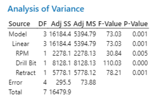
After the experimental runs were completed, the results were analyzed using ANOVA. The initial model included all three main effects and the two-factor interaction terms. The ANOVA results in Table 5 indicate that the interaction terms were not statistically significant (p-value > 0.05). These interactions do not meaningfully explain the observed defects, so they were removed from the model. The ANOVA was recalculated using a reduced model containing only the main effects, as shown in Table 6. All three factors significantly influence the defect seen. The drill bit factor had the largest contribution, accounting for 49.3% of the total variation. Retract rate was the second most influential factor, accounting for 35.1% of the variation, followed by spindle speed, which accounted for 13.8%. The p-values for these factors (0.000, 0.001, 0.005, respectively) reflect strong statistical significance.
Table 5. ANOVA table with all terms.
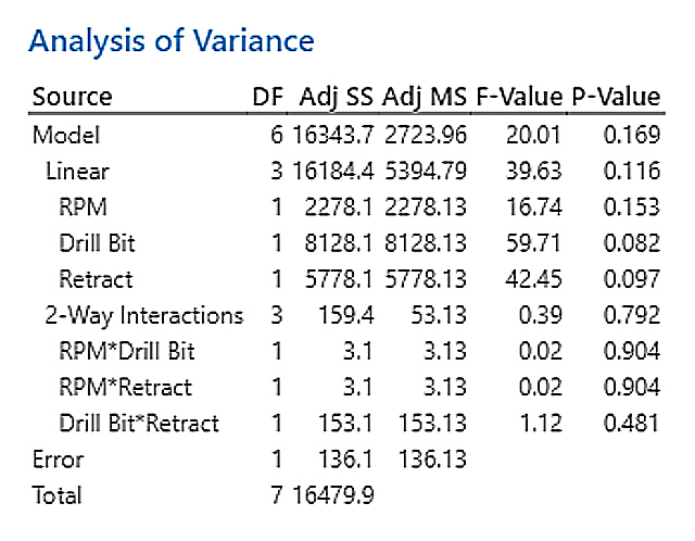
Table 6. ANOVA table with interaction terms removed.
Next, the engineer validates the model by examining the residuals. The probability plot of the residuals approximately follows a straight line. The residuals versus order points fall randomly around the center line, with no recognizable patterns or trends (see Figures 1 and 2). The model summary statistic R-sq indicates that 98.2% of the variation is accounted for by the factors included in the model. The adjusted R-sq is 96.9%, accounting for the number of terms in the model, and provides a more accurate estimation of the model fit. The predicted R-sq of 92.8% indicates that the model provides strong predictability for new observations [2].

Figure 1. Normal probability plot.
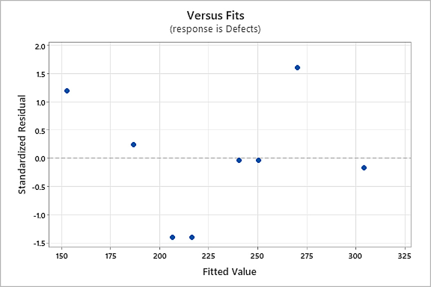
Figure 2. Versus fit plot.
The main effects plots are shown in Figure 3. The slope of each line represents the change in the response as the factor moves from its low level (-1) to its high level (+1). Looking at the main effect plot, the engineer selects the low level (-1) response for each variable: 95K RPM, drill bit type #508, and the retract rate of 550 in/min. Setting the factors at the low levels minimizes the number of defects.
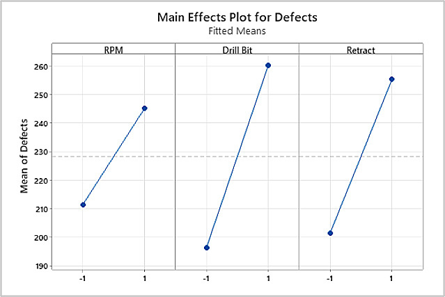
Figure 3. Main effects plot.
Conclusions
While ideal experimental conditions are rarely achievable in production environments, the core statistical principles of DoE remain applicable with proper planning and sound engineering judgment. The example shows that even with limited runs and practical constraints, a 2³ factorial design can identify significant process factors and interactions, providing clear direction for improvement. By combining process knowledge, statistical analysis, and validation techniques (confirmation runs), engineers can ensure conclusions drawn from experimental data are correct, unambiguous, and defensible. Adapting DoE methods to real-world conditions allows organizations to make informed decisions, optimize processes, and drive continuous improvement.
Note: Uyemura’s Lean Six Sigma Black Belts are available to provide introductory design of experiment training. The training presentation covers DoE basics and case studies and takes about 90 minutes to complete. No prior experience is needed, and the case studies are completed using Microsoft Excel. The training is offered virtually or on-site. Please contact your local Uyemura representative for more information.
References
[1] Montgomery, D. C. (2019). Design and analysis of experiments (10th ed.). Wiley, Hoboken NJ.
[2] Valentine, P. (2025). The analysis of variance: Drawing conclusions from data that are correct, unambiguous, and defensible. Printed Circuit Design & Fab, January 2025.
[3] Valentine, P. (2024). How to run a design of experiments. Printed Circuit Design & Fab, September 2024.
[4] Box, G. E. P., Hunter, J. S., & Hunter, W. G. (2005). Statistics for experimenters: Design, innovation, and discovery (2nd ed.). Wiley, Hoboken NJ.
Biography
Patrick Valentine is the Technical and Lean Six Sigma Manager for Uyemura USA. He teaches Six Sigma Green Belt and black belt courses as part of his responsibilities. He holds a Doctorate in Quality Systems Management from Cambridge College and ASQ certifications as a Six Sigma Black Belt and Reliability Engineer. Patrick can be contacted at pvalentine@uyemura.com
Brittany Malin is the Continuous Improvement Manager for Uyemura USA. She holds a Master’s Degree in Quality Systems and Improvement Management from Cambridge College and ASQ certifications as a Six Sigma Black Belt and Reliability Engineer. Brittany can be contacted at bmalin@uyemura.com
April Labonte is the National Technical Manager for Uyemura USA. She holds a Bachelor of Science Degree in Chemical Engineering from the University of California, San Diego. April can be contacted at alabonte@uyemura.com