By Chris Carrillo, April Labonte, Scott Larson, Colin Poedtke, Don Gudeczauskas, and Patrick Valentine
Uyemura International Corporation
Southington CT
Abstract
More understanding of statistical process control (SPC) is needed to implement best practices in PCB manufacturing. The proper use of SPC enables world-class quality "on target with minimal variation." A case study is provided for the micro-etch step of a final finish process.
Introduction
Statistical process control (SPC) is used in manufacturing industries to help reduce process variation and minimize the cost of poor quality (COPQ). Due to the overall complexity of SPC, improper setup and analysis can lead to incorrect conclusions drawn from process data.[1] The need for SPC increases as the electronics industry requires higher reliability and demands less scrap. Statistical process control can keep COPQ low while providing reliable product performance and quality.
Variable selection for SPC applications is critical for collecting valuable information. In the past, classical SPC methods used product attributes such as weight and size to determine process control. As SPC evolved, contemporary methods utilized both product attributes and process variables to monitor where deviations are likely to occur. Ultimately, proper variable selection is vital to bring and keep a process under control.
An eight-step SPC method is used to bring a process under control. The first step is ensuring that the measurement systems are capable of collecting accurate data. Type 1 Gauge and Gauge Repeatability and Reproducibility studies can be conducted to examine the capability of the measurement systems. Experimenters can collect and analyze the data once the measurement systems have been confirmed as capable.
In phase one of data collection, experimenters retrospectively analyze the collected data. An adequate sample size of 20 to 25 (subgroups or individuals) for x-bar or individual charts is collected. Then, the data is plotted, and control limits are computed. Using less than 20 samples produces control limits that are not reliable. The data collected in phase one must be screened before calculating capability indices (Cpk & Ppk).
Before plotting the data in phase one on control charts, the data independence and normality must be confirmed. The lack of independence in the data will underestimate the upper and lower control limits. Non-normal data can influence the tail probabilities, affecting the false alarm rates on control charts. Confirming independence and normality is necessary to draw meaningful conclusions from control charts.[2]
In the 1920s, Dr. Walter A. Shewhart was credited with the invention of control charts while working at Bell Telephone Laboratories.[3] Control charts take advantage of graphing a process variable within upper and lower control limits to determine the stability of a process. Control limits are traditionally set at plus or minus three standard deviations from the mean to ensure that approximately 99-100% of the data will be within these limits. These charts allow trends in a process and out-of-control points to be quickly observed and evaluated.[4]
Range charts (R-charts) and average charts (X-bar or I) are control charts that allow an experimenter to look at the variation and mean of a process, respectively. When R-charts show out-of-control conditions, Lean Six Sigma is essential in reducing the variation in a process. When X-bar or I charts show the mean value of a process is off target, Lean Six Sigma can be used to eliminate the process shift. The use of control charts and Lean Six Sigma collectively aid in bringing a process under control.
Once a process is under control, the stability must be maintained. Process capability indices (Cp, Cpk, Pp, Ppk) numerically define short-term capability and long-term performance.[5] A difference in the short-term capability and long-term performance indicates the presence of assignable causes for process variation. Utilizing capability indices will provide a numeric indicator of process capability and performance.
Once reliable control limits are established, phase 2 of data collection can be used for monitoring the process. A minimum of 100 data points should be sampled to revise control chart limits. Reviewing and revising control chart limits regularly is essential to ensure continuous improvement. Process monitoring is critical for maintaining low variation and minimizing the COPQ.
Experimental Methodology
A control chart is the most common tool used for statistical process control. Control charts can be used to monitor a process and for continuous improvement activities. Statistical process control implementation requires data considerations before charting any variable on a control chart. An eight-step SPC method was utilized to determine process control in this study.
The process under study was the microetch components comprised of hydrogen peroxide and copper concentration. A data set was collected consisting of 95 measurements for each component. The constants used to calculate the SPC chart limits are constructed under the assumption of independence and normality; these must be verified. An autocorrelation function was used to check for independence, and a probability chart was used to verify the normality of the data set.
With independence and normality verified, the data was plotted on a moving range chart. The moving range chart was evaluated for out-of-control points, trends, and patterns. Any out-of-control points were analyzed for assignable causes. After examination, the data was plotted on individual value charts.
Data and control limits were calculated, and individual value charts were created. The individual value chart was evaluated for out-of-control points, trends, and patterns. Any out-of-control points were investigated and analyzed for assignable causes. Various statistical software programs can create control charts and plots.
Minitab® 21 Statistical Software was used to generate all the required plots and charts. These included autocorrelation function plots, probability plots, moving range charts, individual value charts, and capability indices. Using software is the preferred method of performing statistical analysis.
Results
Phase one consisted of collecting 95 data points for the hydrogen peroxide and copper concentration in the microetch bath. The data was graphed on autocorrelation plots utilizing 5% significance limits to verify the assumption of independence. The first three lags should be within the calculated significance limits to confirm independence. The autocorrelation plots for hydrogen peroxide and copper concentration are shown in Figure 1 and Figure 2 respectively.
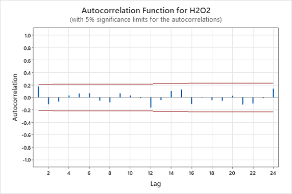
Figure 1. Hydrogen Peroxide Autocorrelation Function.
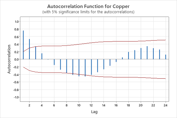
Figure 2. Copper Autocorrelation Function.
The autocorrelation plot confirms the assumption of independence for the hydrogen peroxide. The first three lags in Figure 1 entirely fall within the bounds of the chart. The autocorrelation plot fails the assumption of independence for the copper concentration. The first two lags in Figure 2 violate the 5% significance limits, and there are decreasing waves alternating between positive and negative correlations. The violation of independence will underestimate the upper and lower control limits if plotted on a control chart.
The data was then plotted on probability plots to verify normality. The probability plot utilizes a theoretical normal distribution to compare the data. To verify normality, the data points should form an approximate straight line on the diagonal and yield a p-value greater than 0.05. Probability plots for hydrogen peroxide and copper concentration are shown in Figure 3 and Figure 4 respectively.
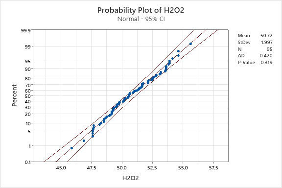
Figure 3. Hydrogen Peroxide Probability Plot.
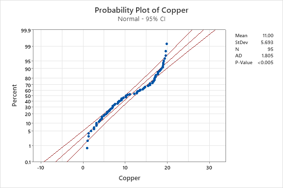
Figure 4. Copper Probability Plot.
The probability plot confirms the assumption of normality for the hydrogen peroxide. Figure 3 shows the data points for the hydrogen peroxide concentration fall near the center line with a p-value significantly greater than 0.05. The probability plot fails the assumption of normality for the copper concentration. Figure 4 shows that the copper concentration does not form an approximately straight line on the diagonal and has a p-value substantially less than 0.05. Non-normal data can influence the tail probabilities, affecting the false alarm rates on control charts.
After evaluating independence and normality for both components, the data was plotted on a moving range chart to visualize the variation. A moving range chart utilizes control limits to determine the absolute difference between points. The data points must fall between the control limits to confirm that the variability is in control. The moving range charts for hydrogen peroxide and copper concentration are shown in Figure 5 and Figure 6 respectively.
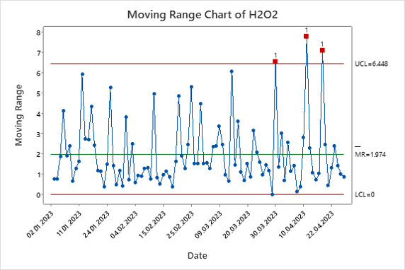
Figure 5. Hydrogen Peroxide Moving Range Chart.
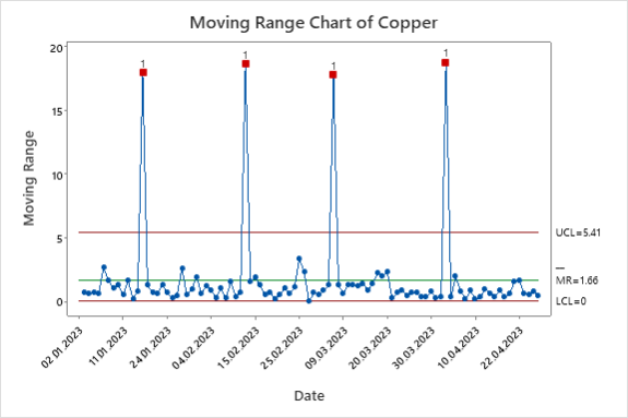
Figure 6. Copper Moving Range Chart.
The moving range charts show that both hydrogen peroxide and copper concentration have points that require further investigation. Figure 5 shows three data points outside of the limits, indicating there may be the need for Lean Six Sigma to reduce the variation in the process. Figure 6 shows a significantly higher level of variation due to probable false points generated from a lack of independence in the copper concentration data. The data was then plotted on an individual chart.
Individual charts calculate the mean, upper and lower control limits at +/- 3σ to indicate whether a component is controlled around the mean. All the points need to fall within these control limits for control to be confirmed. The individual charts for hydrogen peroxide and copper concentration are shown in Figure 7 and Figure 8 respectively.
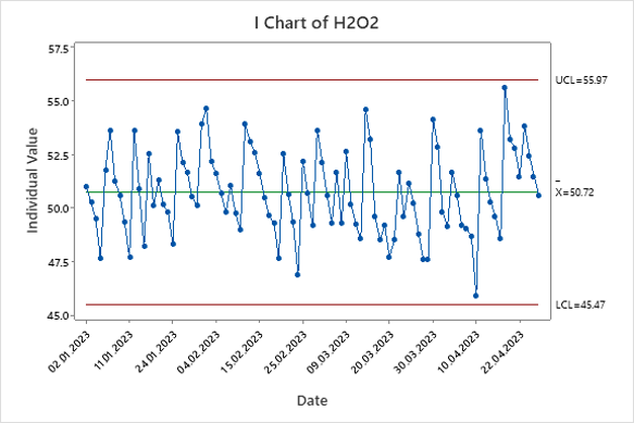
Figure 7. Hydrogen Peroxide Individual Chart.
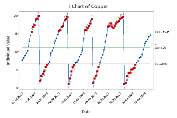
Figure 8. Copper Individual Chart.
The individual chart shows that the hydrogen peroxide concentration data is within the calculated control limits. The computed mean was 50.3 g/L with lower and upper control limits of 45.4 g/L and 55.9 g/L, meeting the hydrogen peroxide specification limit of 40-60 g/L, see Table 1. This indicates that the component is in control with no need to adjust the mean, and the component can continue to be tracked on this chart.
The individual chart shows that the copper concentration exceeds the calculated control limits. The computed mean and control limits for the copper concentration are within the specification of 0-60 g/L, see Table 1, but there are many out-of-control points. These are false points due to a lack of independence in the copper concentration data; the component should not be tracked on this type of control chart.
Table 1. Process Capability Indices for Microetch Components.
| Bath | Component | Mean (g/L) | LSL (g/L) | USL (g/L) | Cpk | Ppk |
|---|---|---|---|---|---|---|
| Microetch | Hydrogen Peroxide | 50.7 | 40 | 60 | 1.55 | 1.77 |
| Copper | 11.0 | 0 | 60; | N/A | N/A |
The process capability and performance indices (Cpk and Ppk) were calculated for hydrogen peroxide as 1.55 and 1.77, respectively, see Table 1. Since the Cpk is nearly equivalent to the Ppk, very little assignable cause variation is present in the process. The optimal target for Cpk and Ppk is greater than 1.33, indicating that the hydrogen peroxide in this study is under excellent control. The indices were not calculated for copper concentration as the component should be plotted on a run chart that does not utilize Cpk and Ppk. Bringing all appropriate components into this level of control will reduce the COPQ and work to achieve world-class quality.
Conclusions
Improper use of SPC is a current problem in the industry. This can result in false alarms impacting COPQ and misusing engineering time and energy. This paper provided an eight-step guideline for proper SPC implementation by analyzing two components of the microetch bath. The following conclusions are provided:
- Hydrogen peroxide concentration was independent and normal and should be tracked on a control chart.
- Copper concentration failed the assumption of independence and normality and should not be tracked on a control chart.
Optimizing the use of SPC can significantly impact the electronics industry. Proper use of SPC will allow engineers to reduce process variation and quickly respond to shifts in the mean. Reducing process variation can lead to an increase in process reliability and a decrease in the COPQ. Understanding the benefits and the proper use of SPC enables world-class quality “on target with minimal variation.”
References
[1] Antony, J. Balbontin, A. Taner, T. (2000). Key ingredients for the effective implementation of statistical process control.
[2] Li Jinmeng, (2021). Application of Statistical Process Control in Engineering Quality Management.
[3] Best, M. Newhauser, D. (2006). Walter A Shewhart, 1924, and the Hawthorne Factory. BMJ Quality & Safety.
[4] Orpana, I. F. (2019). Manufacturing Pharmaceutical Medicines in a Regulated Environment - An Auditor’s Perspective.
[5] Sunadi, S., Purba, H., Saroso, D. (2020). Statistical Process Control (SPC) Method to Improve the Capability Process of Drop Impact Resistance: A Case Study at Aluminum Cans Manufacturing Industry in Indonesia.