By Pat Valentine, PhD
Uyemura International Corporation
Southington CT
Abstract
Nonlinear regression is a powerful statistical tool, but it can be challenging to find the appropriate model and starting parameters. Understanding how to choose the proper model and starting parameters is critical. Linear and nonlinear regression methods are reviewed, and a worked example using electroless nickel immersion gold (ENIG) is provided.
Keywords: nonlinear regression, statistical relationship, Solver, ENIG
Regression analysis utilizes the relationship between quantitative variables to predict one variable from one or more other variables. These relationships are either functional or statistical. Functional relationships have perfect fits. For example, ice cream cones cost $1 each, so that one can buy 10 ice cream cones for $10 or 20 ice cream cones for $20. Statistical relationships typically do not have perfect fits. For example, cholesterol levels and body weight have a non-perfect fit. It is commonly accepted that the term ‘regression’ describes the statistical, not the functional relationship between variables [1].
A regression model is a formal means of expressing the general tendency of a dependent variable (Y) to vary with the independent variable (X) systematically. The independent variable (X) is also referred to as the predictor variable. Box (2007) states, “all models are approximations. Essentially, all models are wrong, but some are useful. However, the approximate nature of the model must always be borne in mind” (p. 414), implying that there are random errors present, hence the non-perfect fit [1, 2]. The expression of the general tendency of a dependent variable (Y) and an independent variable (X) is potent in many different fields.
Regression analysis provides the researcher with three essential purposes: 1) explanation, 2) control, and 3) prediction. Explanation describes the statistical relationship between the dependent variable (Y) and the independent variable (X). Control allows the researcher to set bounds on the independent variable (X) to achieve a controlled output range of the dependent variable (Y). Prediction enables the researcher to answer “what if” questions, e.g., setting the independent variable (X) to a non-common value outside of the control range will likely produce what given output of the dependent variable (Y)? Many times, these three purposes overlap in practice. Regression analysis becomes a unique statistical tool for researchers, process engineers, and others in various fields.
There are many different types of regression models. These models include, but are not limited to, simple linear, multiple linear, nonlinear, orthogonal, calibration, logistic, and Poisson [1, 3]. Simple linear regression is a basic regression model with only one predictor variable (X), and the regression function is linear. Simple linear regression models are considered first-order models. The regression equation has no parameters (β0 intercept or β1 slope) expressed as an exponent, nor are they multiplied or divided by another parameter. The predictor variable (X) appears only in the first-order. Simple linear regression is a good starting point for exploring statistical relationships. Nonlinear regression is a different animal.
Nonlinear regression models are not first-order models. The regression equation has parameters (θ) theta 1, theta 2, etc., that may be expressed as exponents, multiplied or divided by another parameter, etc. The predictor variable (X) may or may not appear in the first-order. When constructing a nonlinear regression model, the model itself must be chosen along with the parameter (θ) starting points (theta 1, theta 2, etc.) [3, 4]. Selecting the model and parameter (θ) starting points (theta 1, theta 2, etc.) requires effort on the researcher's part.
Researchers may not know the actual model tendency of the dependent variable (Y) and the independent variable (X). Without this knowledge, it is challenging to choose a nonlinear model and its starting parameters. In these cases, combining a mechanistic model with an empirical model is a practical approach [3]. Mechanistic models are constructed purely from physical considerations, whereas empirical models are built from data. Small pilot runs can be used for data gathering if no data exists. Combining a mechanistic model with an empirical model provides the best of both worlds. A scatterplot of the data can be constructed and a plausible nonlinear model determined by juxtaposing the scatterplot with graphs of nonlinear models [4]. The most challenging part of nonlinear regression is determining the parameter (θ) theta 1, theta 2, etc., starting points. Microsoft Excel provides a solution [5].
The Solver is an add-in embedded in Microsoft Excel. The Solver is a sophisticated optimization program that enables one to find solutions to complex linear and nonlinear problems. Solver minimizes the sum of the squared difference between data points and the function describing the data [6]. The Solver uses an iterative process, which first requires the researcher to decide upon the initial starting parameter (θ) values for theta 1, theta 2, etc. Solver’s first iteration computes the sum of squares difference. The next iteration involves changing the parameter values by a small amount and recalculating the sum of squares difference. This iterative process is repeated multiple times to achieve the smallest possible value of the sum of squares. A computer algorithm is used for this iterative process.
The researcher can choose from one of three Solver computer algorithms. The three algorithms are 1) Simplex LP Solving Method, 2) Generalized Reduced Gradient (GRG), and 3) Evolutionary Solving Method. The Simplex LP Solving Method can only be applied to linear problems, whereas the Generalized Reduced Gradient and Evolutionary Solving Method can be used for nonlinear problems. The Generalized Reduced Gradient runs faster than the Evolutionary Solving Method, but the algorithm can stop at a local optimum, not necessarily at the global optimum. The Evolutionary Solving Method is based on natural selection theory, which makes it run slower, but it is more robust than the Generalized Reduced Gradient algorithm. Using the Generalized Reduced Gradient Multistart option is a good compromise between speed and robustness.
A worked example:
Electroless nickel immersion gold (ENIG) is the most common printed circuit board final finish in the world. The immersion gold is deposited on the metallic nickel by galvanic corrosion (equation 1). As the nickel becomes covered with gold, the rate of the gold deposition decreases. The optimum gold thickness is typically around 50 nanometers (nm). Too thin of a gold deposit can result in the underlying nickel oxidizing during component assembly resulting in incomplete solder joint formation, i.e., patent defects. Too thick of a gold deposit can cause excessive galvanic corrosion of the underlying nickel resulting in insufficient solder joint reliability, i.e., latent defects.

Equation 1. Galvanic corrosion of metallic nickel by ionic gold.
The ENIG process engineer develops a mechanistic model based on equation one and expects to see the immersion gold plating rate taper off over time. To what extent the immersion gold plating rate tapers off is unknown to the process engineer. Next, the process engineer collects data, under controlled conditions, on gold thickness versus immersion plating time (table 1). Replicates are run to test lack-of-fit during analysis. The process engineer creates a scatterplot (figure 1) and then fits a simple linear regression to the data in table 1 (figure 2).
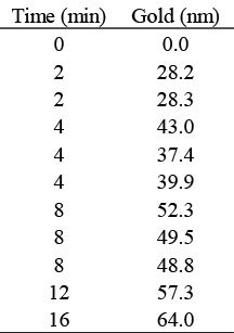
Table 1. Immersion gold versus plating time.
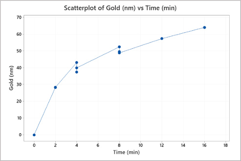
Figure 1. Scatterplot of the data in Table 1.
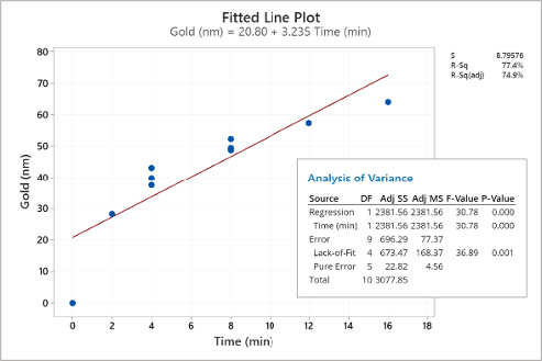
Figure 2. Simple linear regression of the data in Table 1.
The process engineer examines the scatterplot in figure 1. The scatterplot reveals a nonlinear pattern. There appear to be different slopes from zero to two minutes, two to four minutes, four to eight minutes, and eight to 16 minutes. The scatterplot results corroborate the mechanistic model developed from equation 1.
The process engineer examines the scatterplot in figure 1. The scatterplot reveals a nonlinear pattern. There appear to be different slopes from zero to two minutes, two to four minutes, four to eight minutes, and eight to 16 minutes. The scatterplot results corroborate the mechanistic model developed from equation 1. Next, the process engineer examines the simple linear regression seen in figure 2. There is evidence that the simple linear regression fit is inadequate for this empirical model. While the adjusted R-squared value of 74.8% may be acceptable in some circumstances, the simple linear regression reveals a nonlinear pattern. Of more concern is the statistically significant (α = 0.05) p-value of 0.001 for the lack-of-fit indicating the model does not correctly specify the statistical relationship between gold thickness and the plating time; a higher-order term in the model is needed. To further explore the model, the process engineer uses the simple linear regression equation in figure 2 to predict gold thickness at eight minutes, seen in equation 2. The lack-of-fit problem causes the prediction interval for the eight-minute plating time to be broad. The mechanistic and empirical models provide the process engineer enough evidence to warrant fitting a nonlinear regression model.
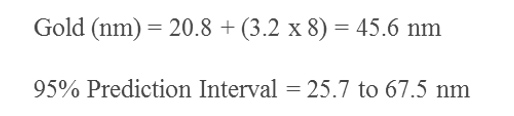
Equation 2. Expected gold thickness with eight a minute dwell time, linear fit.
The process engineer now must find a nonlinear regression function that closely matches the scatterplot in figure 1. Searching through Minitab’s nonlinear regression design catalog, the process engineer finds the Michaelis-Menten function, which appears to be a good fit (figure 3). The Michaelis-Menten function describes the rate of reaction as a function of substrate concentration, in this case, gold thickness versus time. The Michaelis-Menten function aligns well with the mechanistic model developed from equation 1. The Michaelis-Menten function has two parameters (θ), theta1, and theta 2, which need starting values determined. The process engineer now turns to Microsoft Excel Solver.
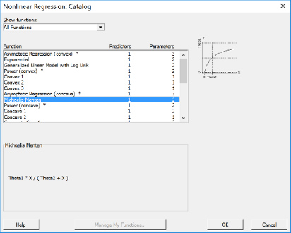
Figure 3. Michaelis-Menten nonlinear function.
The process engineer then builds the Michaelis-Menten function in Microsoft Excel (figure 4). There are five essential inputs needed: 1) fit, 2) residuals, 3) sum of square errors (SSE), 4) theta 1, and 5) theta 2. In figure 4, the input values and mathematical equations are listed in cells A16 through B20. The starting parameters (θ) for theta1 and theta 2 are set at 1.0 for convenience. Next, the process engineer needs to set up Solver.
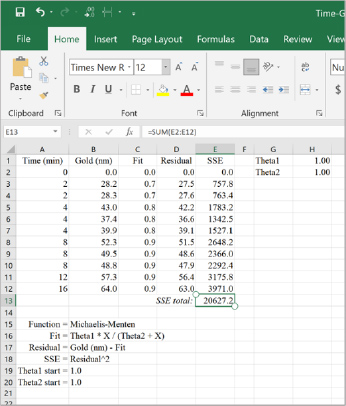
Figure 4. Michaelis-Menten nonlinear function set-up in Microsoft Excel.
There are seven crucial inputs needed for Solver: 1) set objective cell, 2) to value, 3) by changing variable cells, 4) subject to the constraints, 5) make unconstrained variables non-negative, 6) select a solving method, and 7) multistart option. The process engineer inputs the values shown in figures 5 and 6. The ‘objective cell’ is assigned to the total SSE, the ‘to value’ is set to minimize, the ‘changing variable cells’ are assigned to theta 1 and theta 2, constraints are added to the ‘subject to the constraints’ (note: the multistart option requires constraints), ‘make unconstrained variables non-negative’ is unchecked, the ‘solving method’ is set to GRG, and the ‘multistart’ option is checked. The process engineer sets the ‘subject to the constraints' from -100 to +100 to allow wide latitude for the multistart option. Unchecking the 'make unconstrained variables non-negative' allows Solver more freedom in finding a global solution. The process engineer runs Solver, and the results are shown in figure 7.
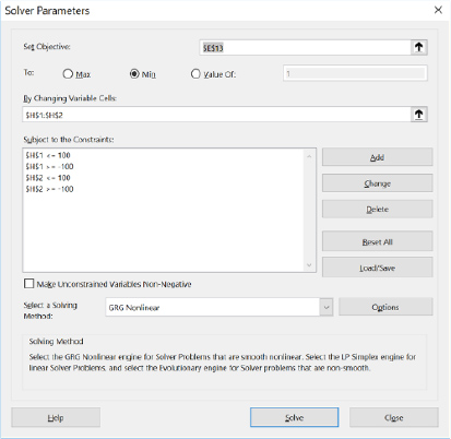
Figure 5. Solver set-up in Microsoft Excel.
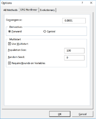
Figure 6. Solver multistart option in Microsoft Excel.
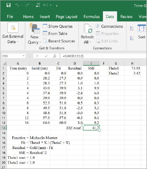
Figure 7. Solver solution.
Solver has found a global solution for this nonlinear problem. The SSE has been minimized to 41.7. Optimum parameters (θ) for theta 1 (73.9) and theta 2 (3.4) have been found. The process engineer now transfers the optimum values of theta 1 and theta 2 into their statistical software package, fits the nonlinear regression, and checks the diagnostics. The nonlinear regression is shown in figure 8, the residual plots are shown in figure 9, and the eight-minute gold thickness prediction using the nonlinear regression equation is shown in equation 3.
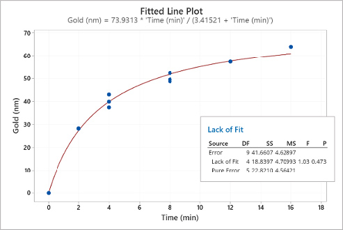
Figure 8. Nonlinear regression of the data in Table 1.
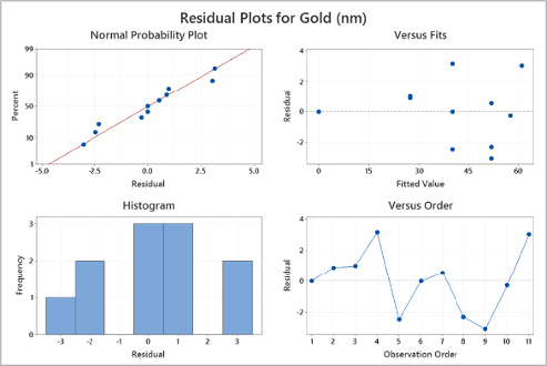
Figure 9. Nonlinear regression residual plots.
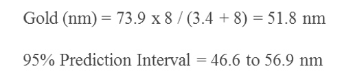
Equation 3. Expected gold thickness with eight a minute dwell time, nonlinear fit.
The nonlinear regression shown in figure 8 fits the data well. The lack-of-fit p-value is 0.473 indicating there is not enough evidence to reject the null hypothesis, i.e., the model correctly specifies the statistical relationship between gold thickness and the plating time. The residual plots shown in figure 9 look normal. The prediction interval for the eight-minute plating time shown in equation 3 is narrow and uniform. The nonlinear regression has been validated and can be used to explain, control, and predict.
Conclusion:
Nonlinear regression analysis is a unique statistical tool for researchers, process engineers, and others in various fields. Nonlinear regression analysis provides three essential purposes: 1) explanation, 2) control, and 3) prediction. In many situations, nonlinear regression can explain mechanistic models better than linear regression. Nonlinear regression has its challenges, though, explicitly choosing the appropriate model and its starting parameters. With nonlinear regression design catalogs, one can use intuition to find a suitable model. Microsoft Excel Solver can easily be used to find the starting parameters. Once a nonlinear regression has been fit, a thorough evaluation of the diagnostics is in order.
References
[1] Neter, J., Kurter, M., Nachtsheim, C., & Wasserman, W. (1996). Applied linear statistical models (4th ed.). United States: McGraw Hill
[2] Box, G., & Draper, N. (2007). Response surfaces, mixtures, and ridge analyses (2nd ed.). Hoboken, NJ: John Wiley & Sons
[3] Ryan, T. (2009). Modern regression methods (2nd ed.). Hoboken, NJ: John Wiley & Sons
[4] Bates, D., & Watts, D. (2007). Nonlinear regression analysis and its applications Hoboken, NJ: John Wiley & Sons
[5] Bowen, W.P., Jerman, J.C. (1995). Nonlinear regression using spreadsheets. Trends in Pharmacological Sciences, 16 (12), 413-417
[6] Brown, A. (2001). A step-by-step guide to nonlinear regression analysis of experimental data using a Microsoft Excel spreadsheet. Computer Methods and Programs in Biomedicine, 65, 191–200
Biography
Patrick Valentine is the Technical and Lean Six Sigma Manager for Uyemura USA. As part of his responsibilities, he teaches lean six sigma green belt and black belt courses. He holds a Doctorate Degree in Quality Systems Management from New England College of Business, Six Sigma Master Black Belt certification from Arizona State University, and ASQ certifications as a Six Sigma Black Belt and Reliability Engineer. Patrick can be contacted at pvalentine@uyemura.com