By Patrick Valentine, PhD
Uyemura International Corporation
Southington CT
Abstract
Measurement is the foundation of quality. We measure for two primary reasons: to make decisions on product quality and as the basis for continuous improvement projects. Statistical tests are powerful tools that help process engineers make better decisions on process improvement projects. The two most common parameters of interest are the mean and standard deviation. The two-sample t-Test and F-test are reviewed, and worked examples using Microsoft Excel are provided. Statistics and probability are explained in colloquial terms.
Keywords: mean, standard deviation, t-Test, F-test, continuous improvement, projects
Introduction
Can we trust our measurement system to give us reliable data? Is it accurate, repeatable, and reproducible? Measurement is the foundation of quality. We measure for two primary reasons: to make decisions on product quality and as the basis for continuous improvement projects. We can engage in continuous improvement projects if we are confident in our measurement systems.
What is the primary skill for which we are on the payroll? It’s our problem-solving skills. Therefore, our function is to solve problems and add value. Dr. Joseph M. Juran stated, "A project is a problem scheduled for solution" [1].
Projects need to be connected to business strategies. Their importance must be clear to the organization. They must have the support and approval of management and be tied to the organization's financials. They need a reasonable scope, typically doable in under six months for Plan Do Check Act (PDCA) or Define Measure Analyze Improve Control (DMAIC) projects. Note that sub-projects may be required first. Project goals must be well-defined, and there must be clear quantitative measures of success. Projects need to be looked at from a statistical point of view.
Statistical thinking views all work as a process and acknowledges variation exists in all processes. Knowledge and management of variation are crucial for sustained success. For any given process, the output (Y) is a function of the inputs (X): Y = f(X1, X2…Xn) + error, where the error is assumed to be random variation.
Statistics and Probability
Statistics is a branch of mathematics that collects, analyzes, interprets, and presents numerical data. It is not merely the science of analyzing data but the art and science of collecting and analyzing data. Statistics are tools to help us; they do not replace the process engineer’s skill and intelligence. Statistics uses hypotheses, experiments, and hypothesis testing.
With hypotheses, a null (H0) and an alternative (H1) are put forth. The null hypothesis states that two population means or variances are equal. The alternative hypothesis is a statement that the two population means or variances are not equal (two-tailed). However, the alternative hypothesis can be either one or two-tailed. The one-tail tests for either inferiority or superiority, while the two-tail tests for parity (not equal). Typically, we test for parity, which tests for both inferiority and superiority.
With hypothesis testing, we either accept the null or alternative hypothesis based on a probability value (alpha). Formally, the null and two-tailed alternative hypotheses for the mean and variance are written as follows:
Mean:
H0 : μ1 = μ2
H1: μ1 ≠ μ2
Variance:
H0 : σ21 = σ22
H1: σ21 ≠ σ22
Alpha defines the test's sensitivity. A value of 0.05 implies that the null hypothesis is rejected 5% of the time when it is, in fact, true. The choice of alpha is somewhat arbitrary, although, in practice, a value of 0.05 is typical. Critical values are cut-off values that define regions where the test statistic is unlikely to lie [2].
Probability is a branch of mathematics that deals with the occurrence of a random event. P-values are expressed from zero to one and are the probability of an event having occurred. The general interpretation of p-values is as follows:
< 0.05 are statistically significant
0.05 ≤ p-value ≤ 0.10 may have a practical difference
> 0.10 is generally considered non-significant
Statistically significant means that the results in the data are not likely explainable by chance alone. Practical difference requires the process engineer to logically determine if the population mean or variance differences have any practical value. Non-significant means the results in the data lie within the limits of chance.
Microsoft Excel Data Analysis ToolPak
The Analysis ToolPak provides tools for statistical data analysis. It offers different kinds of statistical analysis, including t-Tests and F-tests. This enables the exploration and statistical analysis of data without using any external software. ToolPak is, therefore, useful to process engineers working with datasets [3].
To access ToolPak, click Data Analysis in the Analysis group on the Data tab. Suppose the Data Analysis command is not available. In that case, you can load the Analysis ToolPak add-in program by following these steps: 1) Click the File tab, click Options, and then click the Add-Ins category. 2) In the Manage box, select Excel Add-ins and then click Go. Go to Tools > Excel Add-ins in the file menu if you're using Excel for Mac. 3) In the Add-Ins box, check the Analysis ToolPak check box and click OK. If Analysis ToolPak is not listed in the Add-Ins available box, click Browse to locate it. If you are prompted that the Analysis ToolPak is not currently installed on your computer, click Yes to install it [3]. Figure 1 shows some of the analysis tools available in ToolPak.
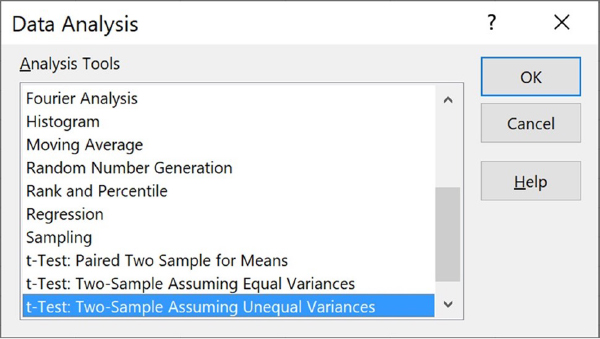
Figure 1. Analysis tools
t-Test
There are three t-Tests to compare means: a one-sample t-Test, a two-sample t-Test and a paired t-Test. The two-sample t-Test is used to determine if two population means are equal. A typical application tests if a new process or treatment is superior to a current one. When comparing two populations, we typically hypothesize that their means are the same. Then, we calculate the test statistic from the data and compare it to a theoretical value from the t-distribution. Depending on the outcome, we either accept the null or alternative hypothesis based on a probability value (alpha). An alpha value of 0.05 is commonly used to accept the alternative hypothesis [2, 4].
Although t-Tests are relatively robust, they are based on several assumptions: The data are continuous, not categorical. The sample data have been randomly sampled from a population. The variance is assumed to be equal (similar in each group). However, this is no longer an issue with computers, and we can default to test with unequal variances. The distributions are approximately normal. For two-sample t-Tests, we must have independent samples. If the samples are not independent, then a paired t-Test may be appropriate [2, 4].
After evaluating independence and normality for both components, the data was plotted on a moving range chart to visualize the variation. A moving range chart utilizes control limits to determine the absolute difference between points. The data points must fall between the control limits to confirm that the variability is in control. The moving range charts for hydrogen peroxide and copper concentration are shown in Figure 5 and Figure 6 respectively.
Table 1 provides a data set, Table 2 shows the ToolPak two-sample t-Test (assuming unequal variances) output, and Table 3 gives the output explanations.
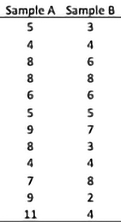
Table 1. Data, Sample A and Sample B
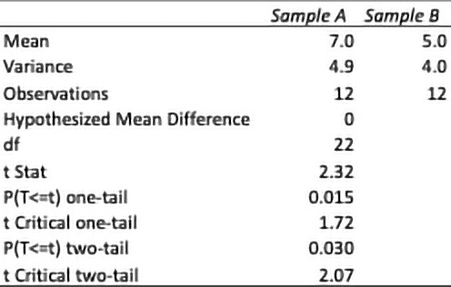
Table 2. t-Test: two-sample assuming unequal variances
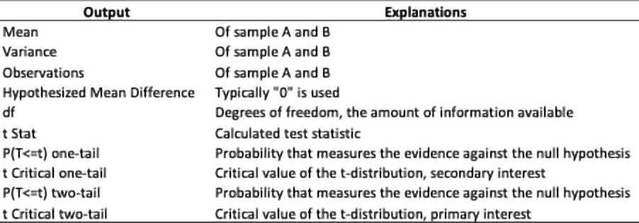
Table 3. t-Test output explanations
F-test
The F-test is used to test if the variances of two populations are equal (we need to work in units of variance when calculating F statistics; variance = standard deviation squared [σ2]). A typical application tests if a new process or treatment is superior to a current one. When comparing two populations, we typically hypothesize that their variances are the same. Then, we calculate the test statistic from the data and compare it to a theoretical value from the F-distribution. Depending on the outcome, we either accept the null or alternative hypothesis based on a probability value (alpha). An alpha value of 0.05 is commonly used to accept the alternative hypothesis [2, 4].
Although F-tests are relatively robust, they are based on several assumptions: The data are continuous, not categorical. The sample data have been randomly sampled from a population. The distributions are approximately normal, free from severe skewness and outliers. The samples are independent [2, 4].
The number of observations should be ≥ 12 for each sample. With ≥ 12 observations, precision is maximized by decreasing the width of the confidence interval of the variance. This provides enough power for the F-test. Power is the conditional probability that you will avoid a Type II error, accepting the null hypothesis when, in fact, it's false.
The data set in Table 1 is used here. The ToolPak two-sample F-test output is shown in Table 4, and the output explanations are given in Table 5. Of particular note in Table 4 is that only the one-tail output exists. Because our interest is in parity, we want the two-tail output. All we need to do is double the one-tail p-value output: 0.370 X 2 = 0.740.
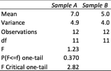
Table 4. F-test: two-sample
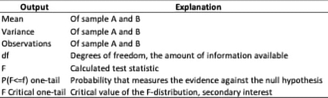
Table 5. F-test output explanations
A Worked Example
A young engineer is undertaking an inner layer improvement project. The goal is to achieve World-Class Quality, "on target with minimal variation," by reducing opens. The engineer designs an experiment: the current process and a new process (see Table 6).
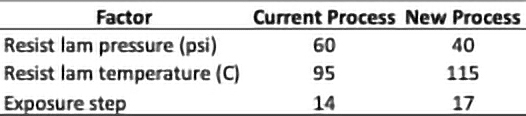
Table 6. Inner layer experiment
The process engineer then collects data for each process over 12 consecutive days. She processes 100 inner layers through each process and records the total count of opens for that day (see Table 7). Note that the same job number is used for each process to minimize noise (uncontrollable factors).
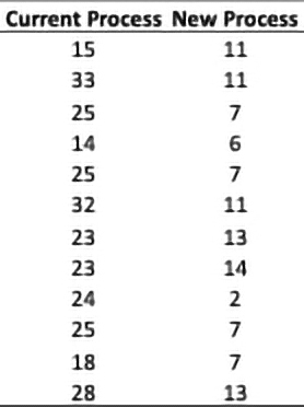
Table 7. The count of the inner layer opens
The next step is the analysis. The process engineer wants to evaluate both the mean and standard deviation. The first step is the two-sample t-Test. Using the ToolPak, the process engineer loads the data for analysis (see Figure 2). The output is shown in Table 8.
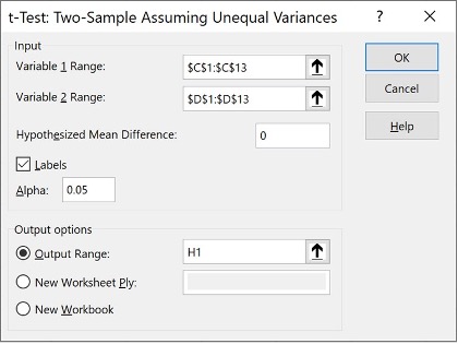
Figure 2. Two-sample t-Test assuming unequal variances
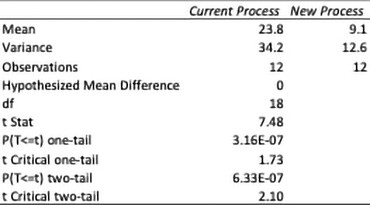
Table 8. Two-sample t-Test output
Discussion: The mean values for opens for the current and new process are 23.8 and 9.1, respectively. The two-tailed p-value is significantly lower than the alpha value of 0.05. With an alpha value of 0.05, there is only a 5% chance of rejecting the null hypothesis when it is, in fact, true (the population means are equal). The process engineer concludes that the means are statistically significant; the results in the data are not likely explainable by chance alone. The new process has statistically proven to improve inner layer yields.
Next, the process engineer analyzes the variance using the two-sample F-test. The process engineer loads the data into ToolPak for analysis (see Figure 3), and the output is shown in Table 9.
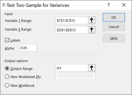
Figure 3. Two-sample F-test
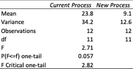
Table 9. Two-sample F-test output
Discussion: The variance values for opens for the current and new process are 34.2 and 12.6, respectively. Because the p-value is for a one-tailed test, the process engineer converts the p-value to a two-tailed test by multiplying the p-value by two (0.057 X 2 = 0.114). The p-value is greater than the alpha value of 0.05. The process engineer concludes that the variances are not statistically significant; the results in the data are likely explainable by chance. Because the p-value is greater than 0.10, the variance is considered non-significant. However, the process engineer must logically determine if the population variance differences have practical value. A second improvement project could be undertaken to reduce the variation.
Conclusions
Achieving World-Class Quality, "on target with minimal variation," requires continuous improvement projects. The two most common project parameters of interest are the mean and standard deviation. Statistical tests are an integral part of analyzing those projects. The two-sample t-Test and F-test are practical statistical tools for analyzing the mean and standard deviation. However, statistics are tools that can help us; they do not replace the process engineer’s skill and intelligence. Microsoft Excel Data Analysis ToolPak is a ubiquitous and convenient software for these analyses. Ultimately, the process engineer's function is to solve problems and add value.
References
[1] Heagney, J. (2016). Fundamentals of Project Management, 5th Edition. New York: AMACOM
[2] NIST Engineering Statistics Handbook. (2012). http://www.itl.nist.gov/div898/handbook/
[3] Retrieved from support.microsoft.com
[4] JMP Software
Biography
Patrick Valentine is the Technical and Lean Six Sigma Manager for Uyemura USA. He teaches Six Sigma Green Belt and black belt courses as part of his responsibilities. He holds a Doctorate in Quality Systems Management from Cambridge College and ASQ certifications as a Six Sigma Black Belt and Reliability Engineer. Patrick can be contacted at pvalentine@uyemura.com