By Pat Valentine, PhD
Uyemura International Corporation
Southington CT
Abstract
Design of experiments (DoE) is an efficient method for planning experimental tests so that the data obtained can be analyzed to produce valid and objective conclusions. Designed experiments are commonly used for product and process design, development, and improvement. This paper reviews the history of designed experiments, experimental design, common design of experiments, and experimental steps.
Keywords: design of experiments, scientific method
Introduction
Aristotle (384 – 322 BC) laid the foundation for the scientific method. At the beginning of the 19th century, science was established as an independent and respected field of study, and the scientific method was embraced worldwide. The scientific method is a five-step process. These five steps are 1) make observations, 2) propose a hypothesis, 3) design and conduct an experiment, 4) analyze the data, 5) accept or reject the hypothesis, and, if necessary, propose and test a new hypothesis. Early experiments were one-factor-at-a-time (OFAT). These designs would vary only one factor or variable at a time while keeping the others fixed. But in 1922, things changed.
In 1922 – 1923, R. A. Fisher (see Figure 1) published essential papers on designed experiments and their application to the agricultural sciences. Fisher is revered as the godfather of modern experimentation. Then, in 1932–1933, the British textile and woolen industry and the German chemical industry began using designed experiments for product and process development. In 1951, Box and Wilson started publishing fundamental work using designed experiments and response surface methodology (RSM) for process optimization. Their focus was on the chemical industry. The applications of designed experiments in the chemical industry began to increase. From 1975 through 1978, books on designed experiments geared toward engineers and scientists began to appear. In the 1980s, various organizations adopted experimental design methods, including electronics, aerospace, semiconductor, and the automotive industries. Taguchi's methods of designed experiments first appeared in the United States. In 1986, statisticians and engineers visiting Japan saw firsthand the extensive use of designed experiments and other statistical methods. During the early 1970s through the late 1980s, proprietary design of experiment software began to emerge (Minitab, JMP, and Design Expert). In 2011, Jones and Nachtsheim introduced the definitive screening design of experiments [1, 2].

Figure 1. Sir Ronald Fisher
In the 1950s, product and process improvement designed experiments were introduced in the United States. The initial use was in the chemical industry, where the power of designed experiments became widely harnessed. This is one reason why the U.S. chemical industry has remained one of the most competitive in the world.
The spread of designed experiments outside the chemical industry was relatively slow until the late 1970s and early 1980s. Then, many Western companies learned that their Japanese competitors had been systematically using designed experiments since the 1960s. Japanese companies used designed experiments for new process development, process improvement, and reliability improvements. This discovery catalyzed extensive efforts to introduce designed experiments in the engineering field and academic engineering curricula.
Experimental Design
With an experiment, we deliberately change one or more input process factors to observe the changes' effect on the response variables. An application example is shown in Figure 2. Design of experiments is an efficient method for planning experiments so that the data obtained can be analyzed to produce valid and objective conclusions. Design of experiments begins with determining the experiment's objectives; designed experiments are commonly used for product and process design, development, and improvement. Process factors and levels are then selected for the study. Knowledgeable Six Sigma Black Belts and process engineers understand and harness the power of DoE.
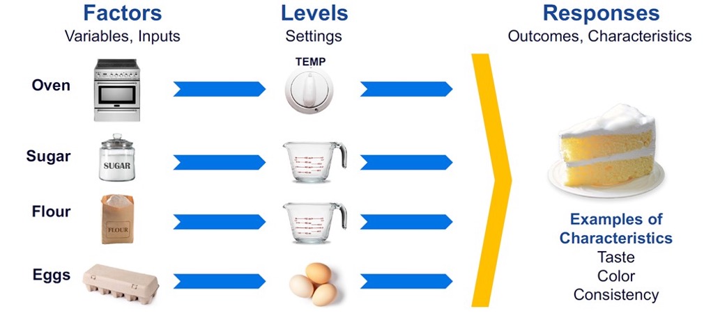
Figure 2. Application of design of experiments
An experimental design is the creation of a detailed experimental plan before experimenting. Properly chosen experimental designs maximize the information that can be obtained for the given amount of experimental effort. Two-level factorial and fractional factorial designs are typically used for factor screening and process characterization. The most common model fit to these designed experiments is a linear form. Response Surface designs are typically used to find improved or optimal process settings, troubleshoot process problems and weak points, or make a product or process more robust against external and non-controllable influences. The most common model fit to these designed experiments is a quadratic form.
Experiments commonly need to account for some uncontrolled factors (noise) that can be discrete (different shifts or operators, etc.) or continuous (ambient temperature or humidity, etc.). Noise factors may be identified or unidentified and can change during the experiment. The presence of noise factors is called a Black Box process (see Figure 3).
Noise factors can be tolerated when they are managed correctly and disastrous when they are not. Managing noise factors is accomplished by randomization.
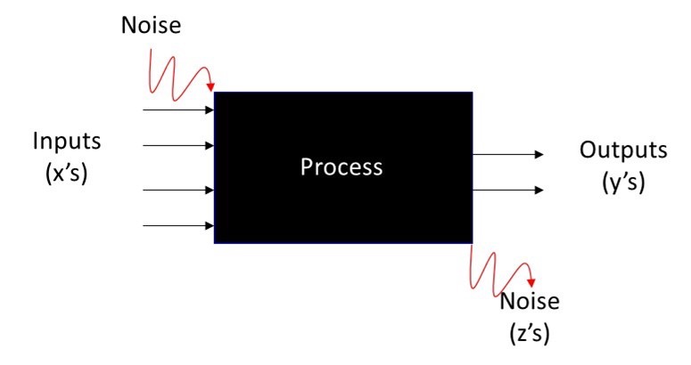
Figure 3. Black Box process model schematic
Randomization is a schedule for running DoE combinations so that the conditions in one run do not depend on the conditions of the previous run, nor do they predict the conditions in the subsequent runs. The importance of randomization cannot be overemphasized. It is necessary if conclusions drawn from the experiment are to be correct, unambiguous, and defensible [3].
The design of experiment resolution is a term that describes the degree to which estimated main effects are confounded with estimated 2-level interactions, 3-level interactions, etc., and is commonly identified in Roman numerals. If some main effects are confounded with 2-level interactions, the resolution is III. Full factorial designs have no confounding and have a resolution of "infinity." A resolution V design is excellent for most purposes, and a resolution IV design may be adequate. Resolution III designs are functional as economical screening designs [3].
Common Design of Experiments
ANOVA: The analysis of variance design has two primary subcategories. The One-way supports one numeric or categorical factor at ≥ 2 levels, and the two-way supports two numeric or categorical factors at ≥ 2 levels. These designs are extensions of the t-test.
Combined designs: An excellent choice when working with mixtures in combination with categorical and continuous factors. These designs support factors at > 3 levels and identify significant main effects, all interactions, and quadratics. You can add constraints to your design space, for instance, to exclude a particular area where responses are known to be undesirable.
Definitive Screening designs: Incorporate mid-levels for each factor, allowing individual curvature estimation. They efficiently estimate main and quadratic effects for no more and often fewer trials than traditional designs. They can be augmented to support a response surface model. They are an excellent choice for screening multiple factors.
F-test: One numeric or categorical factor at two levels. Used to test if the variances of two populations are equal. A typical application tests if a new process or treatment is superior to a current one.
Full and Fractional Factorials 2k designs: Numeric and categorical factors at two levels. Estimation of main effects and interactions, and can detect curvature by adding center points. Full factorials measure responses at all combinations of the factor levels. In contrast, fractional factorials measure responses for a subset of the original full design. This reduces the total runs, but the tradeoff is design confounding.
General Factorial designs: Numeric and categorical factors at ≥ 2 levels. Identifies main effects, all interactions, and quadratics. Measures responses at all combinations of the factor levels. These designs become very large with ≥ 5 factors and are generally not cost or time-efficient.
Irregular Fraction designs: Numeric and categorical factors at ≥ 2 levels. Estimation of main effects and two-factor interactions. These are resolution V designs with unusual fractions like 3/4 or 3/8. They are also known as space savers, reducing runs by 25%. These designs are a great choice as they reduce runs and are still resolution V.
Minimum Run Resolution IV and V designs: Numeric and categorical factors at ≥ 2 levels. Estimation of main effects and some interactions. Suitable for screening, designed for ≥ 5 factors. It's a good choice if interactions are unlikely..
Mixture designs: Components from 2-50, expressed as either proportions (from 0-1) or values (lbs, ounces, grams). Designs include Simplex Centroid or Lattice and Extreme Vertices. Design points are arranged uniformly (lattice) over a simplex (a generalization of a triangle or tetrahedron to an arbitrary dimension). Can add points to the interior of the design space.
OFAT: One-factor-at-a-time designs vary only one factor at a time while keeping the others fixed. OFAT are useful in some situations but should not be the first choice. They become invaluable with complex systems and extremely hard-to-change factors, such as varying the copper level in an electroplating via fill tank. However, randomization is impossible. OFAT are best analyzed with partial least squares regression.
Optimal designs: Numeric and categorical factors at ≥ 2 levels. These designs are known as alphabet optimality. Designs are generated based on a particular optimality criterion (D, G, A, E, I, L, C, S) and are generally optimal only for a specific statistical model. D and I-optimal are the most common. Optimality is either maximized or minimized. Optimal designs are excellent for regions of constraints and costly runs. Designs are not orthogonal by nature.
Plackett-Burman designs: Numeric and categorical factors at two levels. Can estimate main effects. Good for screening ≥ 7 factors. Useful for ruggedness testing (validation) where you hope to find little or no effect on the response due to any factors [4]. The 12-run design has a unique attribute: there is a weak correlation among the factors, so confounding is minimized, and the interactions are uniformly dispersed over all the experimental runs.
Randomized Blocked Designs (RBD): Supports two factors at ≥ 2 levels, but interest lies in only one factor. Used when a noise factor is known and controllable, but you do not intend to make claims about the differences between the levels of the noise factor. Typical noise factors are raw material lot numbers, locations, plants, operators, etc.
Response Surface Method (RSM): Primarily numeric factors at ≥ 3 levels, but categorical factors can be added. Identifies main effects, all interactions, and quadratics. The RSM family includes Central Composite, Box-Behnken, and 3k designs. They can become enormous with ≥ 4 factors.
Split-plot designs: Numeric and categorical factors at two levels. Estimation of main effects and two-factor interactions. Excellent designs for hard-to-change factors (HTC). Hard-to-change factors are challenging to randomize due to time or cost. These designs range from resolution III on up.
t-Test: One numeric or categorical factor at two levels. Used to test if two population means are equal. A typical application tests if a new process or treatment is superior to a current one.
Experimental Steps
There are six fundamental steps with DoE: 1) state the problem, define the objectives, 2) design the experiment, 3) run the experiment, 4) analyze the experiment, 5) confirmation runs and Ppk, and 6) report and recommendations.
State the Problem, Define the Objectives
Do we have a clear understanding of the problem? Why are we doing this DoE? What is the desired outcome for the response? Typically, either Better (e.g., reliability, aesthetics), Faster (e.g., drying, curing), Cheaper (e.g., lower cost, less reaction time), or Positive Outcome (e.g., marketing, advertising). A team discussion best determines the objectives of an experiment. The group should discuss the key objectives and which ones are "nice but not necessary." All of the objectives should be written down.
Design the Experiment
Successful experimental designs incorporate both process knowledge and sound statistical procedures. Process knowledge is invaluable in the design stages and in interpreting the results. Experimental design is commonly an iterative approach – rarely does one run a single large comprehensive DoE in which final conclusions are made. Choose factors and reasonable ranges for each. Determine appropriate responses and how to measure them. Select a design, know your pros and cons, and review runs. Check the factor settings for impractical or impossible combinations. The choice of an experimental design depends on the experiment's objectives and the number of factors to be investigated. Generally, we use resolution III designs to screen several main factors and resolution IV or above for interactions. A DoE design guide is shown in Figure 4.
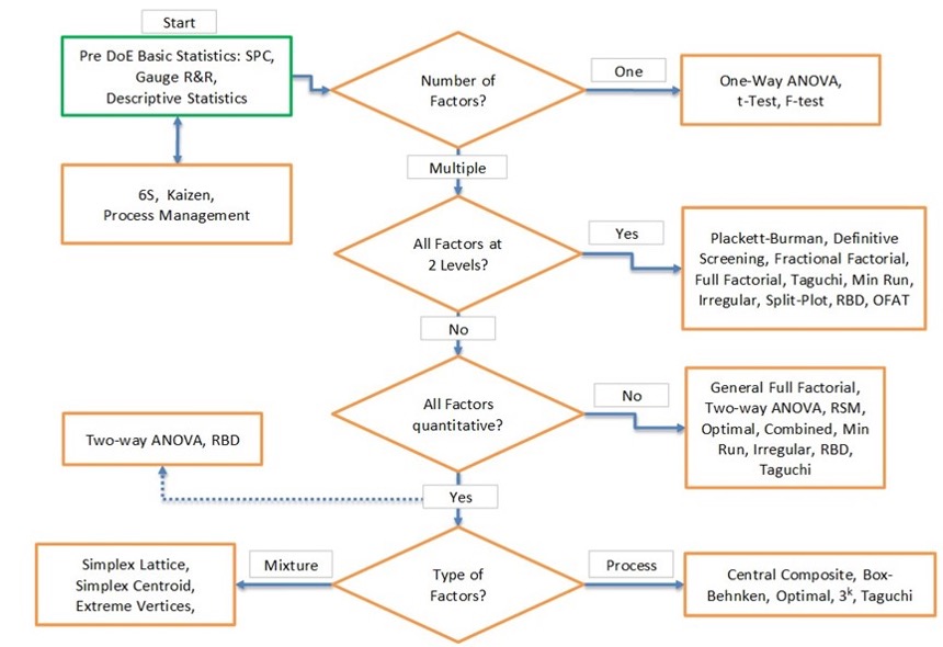
Figure 4. DoE design guide
Run the Experiment
There are five cardinal rules: 1) Be involved, 2) Keep an eye on everything, 3) Don’t guess or make assumptions, 4) Block out known sources of variation, and 5) Randomize the runs. Noise variables can confound one or more of the study variables; an uncontrolled and unobserved variable that changes during the experiment and might affect the response. Randomization helps protect against noise variables but doesn't compensate entirely for their effect. Randomization will desensitize an experiment to the effects of noise variables and more accurately predict the real differences between treatment means.
Analyze the Experiment
Multiple steps are required when systematically analyzing experimental data (see Figure 5). Errors can be introduced into an experiment in four ways: 1) A significant factor(s) was/is missed, 2) There is an error in your measurements, 3) Unknown noise factor(s) were present during experimentation, 4) Excessive variation (inherent in the process itself – lack of statistical process control, poor controls during experimentation, etc.).
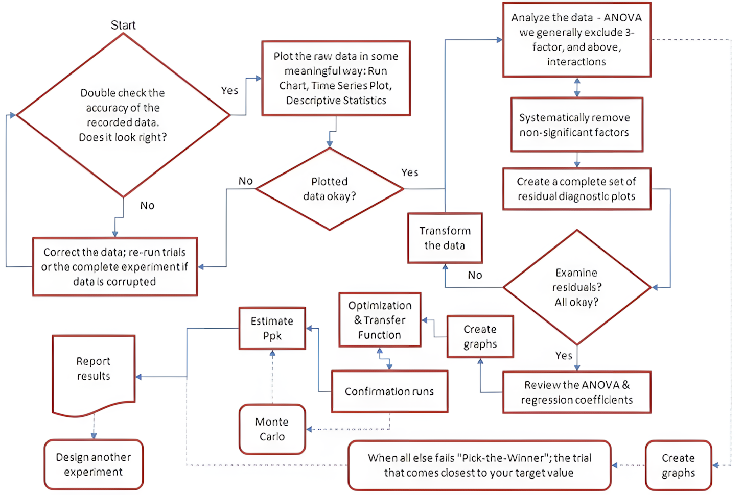
Figure 5. DoE analysis flowchart
Confirmation runs, and Ppk
When the experiment analysis is complete, one must verify that the predictions are reasonable. This is accomplished through confirmation runs. These runs ensure nothing has changed and the response values are close to their predicted values. The number of runs depends on the cost per run, the time per run, product reliability concerns, and whether or not the runs will generate production (saleable product). As a rule of thumb, 4 to 20 runs are typical. Still, you should do enough runs to confidently estimate the mean and standard deviation.
The Ppk index provides an estimate of the long-term actual performance. Actual performance is based on the process average and the standard deviation. This overall variation is comprised of both common cause and assignable cause variation. The Ppk index estimates the total variation and accurately tells us "what the customer feels."
Report and Recommendations
Put your recommendations upfront. State them clearly and concisely and back up your reasons. Provide the Ppk for the confirmatory runs. Review the DoE design and analysis. Know your audience: Provide clear and easy-to-follow statistics, an ANOVA table, regression coefficients, graphs, pictures, etc.
Conclusions
Design of experiments are commonly used for product and process design, development, and improvement. An experimental design is the creation of a detailed experimental plan before experimenting. There are dozens of different designed experiments; choosing the right one is a mix of experience, process and statistical knowledge. There are six fundamental steps to creating, running, and analyzing a design of experiments. Knowledgeable Six Sigma Black Belts and process engineers understand and harness the power of DoE.
References
[1] Montgomery, D. (2009). Introduction to Statistical Quality Control, 6th Ed. United States: John Wiley & Sons.
[2] Jones, B. & Nachtsheim, J. (2011). Definitive Screening in the Presence of Second-Order Effects. Journal of Quality Technology, Vol. 43, No. 1, January
[3] NIST Engineering Statistics Handbook. (2012). http://www.itl.nist.gov/div898/handbook/
[4] ASTM Standard E 1169
Biography
Patrick Valentine is the Technical and Lean Six Sigma Manager for Uyemura USA. He teaches Six Sigma Green Belt and black belt courses as part of his responsibilities. He holds a Doctorate in Quality Systems Management from Cambridge College and ASQ certifications as a Six Sigma Black Belt and Reliability Engineer. Patrick can be contacted at pvalentine@uyemura.com