By Pat Valentine, PhD
Uyemura International Corporation
Southington CT
Abstract
Process yield statistics are powerful tools that help an organization see how defects impact their scrap, rework, warranty, and customer satisfaction. It can be challenging to choose the appropriate statistics and starting parameters. Understanding the fundamental basics is critical for process improvement. Process yield statistics and distributions are reviewed, and a worked example is provided.
Keywords: first-time yield, rolled throughput yield, Poisson and binomial distributions, attribute charts, hidden factory
Introduction
The costs of poor quality include all expenses incurred for not making or providing a perfect product the first time, including scrap, rework, re-purchasing raw materials, labor, and inventory [1]. Companies operating at a three-sigma quality level can spend about 25% of their annual sales remediating poor quality costs [2]. Other estimates put the costs of poor quality in the range of 25 to 40% [3]. Poor quality can destroy a company.
Unexpected product failures significantly increase selling, general, and administrative (SG&A) costs and lead to increases in inventories and fixed assets required to support operations. These indirect costs erode profitability more than those directly attributable to warranty claims processes. Product recalls negatively impact businesses financially and result in adverse publicity. Customers expect printed circuit boards to meet their specifications.
An internal Motorola study found that units reworked in production often encountered problems during early customer use, even though the defects identified were corrected during production. Rework can frequently stress a unit non-standardly and predispose a product to early failure [4]. Denson found a similar occurrence in semiconductor manufacturing, where the reliability of computer chips was statistically correlated with the die yield [5]. These studies suggest that circumstances in detecting and reworking defects in some units may produce undetected damage on other units. When delivered to customers, these weaknesses often contribute to early failures.
Defects are any items that exhibit a departure from specifications. A defect does not necessarily mean that the product cannot be used; it only indicates that the product result is not as intended. In essence, defects refer to quality characteristics. Generally, the count of defects is assumed to follow a Poisson distribution.
Defectives are units that are considered completely unacceptable for use. Each unit is deemed defective or not–there are only two choices. In essence, a defective unit refers to the overall product. Generally, the count of defective units is assumed to follow a binomial distribution.
A count of defects usually contains more information than a count of defective units. When either number can be obtained with approximately the same effort, using counts of defects rather than defective units is generally preferable. However, defect rates are rarely high enough in most production processes to create any substantive difference between counts of defects and defectives. There are a few exceptions to this [6].
The frequency of first-time yield (FTY) monitoring depends on your specific needs and your system's quality standards. Generally, FTY should be checked as often as your system allows. This could be a day, week, month, or any other time frame that fits your production cycles and allocated resources and allows for meaningful analysis.
Yield Statistics and Discrete Distributions
Statistics is a branch of mathematics that collects, analyzes, interprets, and presents numerical data. Statistics is not merely the science of analyzing data but the art and science of collecting and analyzing data. Statistics are only tools to help us; they do not replace the process engineer’s skill and intelligence. Statistics are fundamental for process improvement activities.
First-time yield (FTY) is the percentage of units that pass through an individual process without defects. Rolled throughput yield (RTY) estimates the probability that a unit passes through all process steps defect-free. The FTY and RTY are easy to compute, and the RTY is highly correlated with scrap, rework, warranty costs, and customer satisfaction.
A discrete distribution is a probability distribution that depicts the occurrence of discrete (individually countable) outcomes, such as 1, 2, 3, yes, no, true, or false. For the most part, discrete distributions use up to two parameters: 1) probability of an event, p, and 2) number of trials, n. A few exceptions exist to this notation, the Poisson distribution being one of them.
A Poisson random variable is a discrete random variable representing the count of independent events occurring per unit of time, space, or product. Poisson random variables may represent defects per inner layer (I/L), outer layer (O/L), etc. The Poisson distribution is one of the simplest distribution models, with a single parameter lambda (λ) representing the mean count of events [7, 8].
A binomial random variable is a discrete random variable representing the count of defective units in a sample of n independent trials when the probability of any defective unit is p. Binomial random variables may represent defective units due to shorts, opens, voids, etc. The binomial distribution is used when there are precisely two mutually exclusive trial outcomes, "pass" or "fail ."The binomial distribution is a simple distribution model with two parameters: n number of trials and p probability of “passing” with 0 ≤ p ≤ 1[7, 8].
Statistical Tools for Analyzing and Monitoring Defects and Defectives
We use analyses based on a Poisson probability model to evaluate defects. These analyses evaluate the rate of defects in a process. Standard statistical tools include the C Chart: used to monitor the number of defects where each unit can have multiple defects. You should use a C chart only when your subgroups are the same size. U Chart: used to monitor the number of defects per unit, where each unit can have multiple defects and various subgroup sizes. U Chart Diagnostic: used to test for overdispersion or underdispersion in your defects data; note, overdispersion and underdispersion are mutually exclusive. Overdispersion can cause a traditional U chart to show increased points outside the control limits. Underdispersion can cause a conventional U chart to show too few points outside the control limits. The Laney U' chart adjusts for these conditions. Poisson Capability Analysis determines whether the defects per unit (DPU) rate meets customer requirements [9].
We use analyses based on a binomial probability model to evaluate defectives. These analyses evaluate the proportion of defectives in a process. Standard statistical tools include the P Chart: used to monitor the proportion of defective units where each unit can be classified into one of two categories: pass or fail, and with various subgroup sizes. P Chart Diagnostic: used to test for overdispersion or underdispersion in your defectives data; note, overdispersion and underdispersion are mutually exclusive. Overdispersion can cause a traditional P chart to show increased points outside the control limits. Underdispersion can cause a conventional P chart to show too few points outside the control limits. The Laney P' chart adjusts for these conditions. NP Chart: used to monitor the number of defective units; each unit can be classified into one of two categories: pass or fail, and has various subgroup sizes. Note: if your subgroup sizes are not equal, the center line will not be straight. Binomial Capability Analysis: used to determine whether the percentage of defective units meets customer requirements [9].
A Worked Example
A young engineer understands the importance of yield statistics concerning customer satisfaction and continuous process improvement. Unfortunately, she has no data on defects. Still, she does have limited data on defective units processed through the inner-layer (I/L), making holes conductive (MHC), and outer-layer (O/L) processes. She reviews the last eight weeks of production data as a starting point and calculates the FTY and RTY statistics, see Table 1. Because we are working with defective units, she will use statistical analyses based on a binomial probability model.
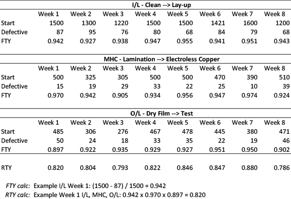
Table 1. Eight weeks of production data.
The engineer checks for the presence of overdispersion or underdispersion using the P Chart Diagnostic test for the inner-layer (I/L), making holes conductive (MHC), and outer-layer (O/L) processes. The data points (Defective proportions) should align close to a diagonal line, indicating a good fit. The origin of the red diagonal line comes from the binomial distribution parameters n and p. All three FTY diagnostic tests lack evidence to support overdispersion or underdispersion. Figure 1 shows the P Chart Diagnostic test for the I/L process. The variation ratio (104.4%) is significantly less than the 95% upper limit of 243.7%, corroborating no overdispersion.
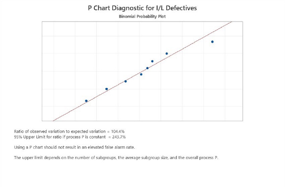
Figure 1. P Chart Diagnostic test of I/L defectives.
Next, the engineer generates P Charts for the inner-layer (I/L), making holes conductive (MHC) and outer-layer (O/L) processes. The center line is the average proportion of defectives. The control limits are set at a distance of three standard deviations above and below the center line and vary due to unequal sample sizes. All points are in control. Figure 2 shows the P Chart for the I/L process.
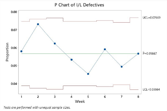
Figure 2. P Chart of I/L defectives.
Next, the engineer generates Capability Analysis reports for the inner-layer (I/L), making holes conductive (MHC) and outer-layer (O/L) processes. The report displays four graphs: 1) P Chart, 2) Rate of Defectives, 3) Cumulative % Defective, and 4) Histogram. Figure 3 shows the Capability Analysis report for the I/L process.
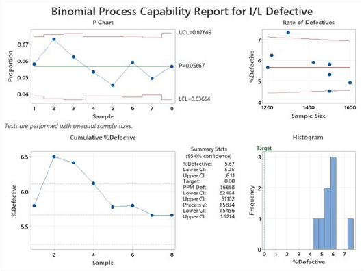
Figure 3. Capability Analysis report for the I/L defectives.
There is much information contained in the report, and the process engineer extracts and infers the following:
P Chart: The I/L process %defective is stable and in control.
Rate of Defectives: The data fall randomly about the center line; the probability of a defective item is constant across different sample sizes. The data follow a binomial distribution.
Cumulative % Defective: The %defective is stabilizing, shown by a flattening of the plotted points along the mean %defective line. There are enough samples for a stable estimate of the %defective.
Histogram: The peak represents the most common values and approximates the center of the %defectives, about 6%. The spread varies about 3%. The engineer realizes histograms need at least 50 data points for unambiguous interpretation.
Finally, the engineer wants to chart the RTY. She decides that a Run Chart is the most straightforward and efficient method. Run Charts expose patterns or trends that indicate the presence of special-cause variation [9]. The engineer noticed that the RTY trended up from week three through week seven and then dropped sharply in week eight. Investigation is warranted to determine what happened; see Figure 4.
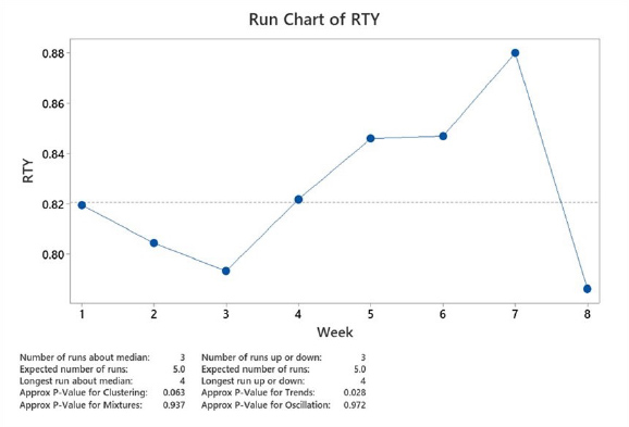
Figure 4. Run Chart of RTY.
Unlike the FTY, the RTY exposes the “hidden factory” [10]. The term “hidden factory” refers to unseen activities outside the normal processes that occur when a defect is discovered. These unseen activities add labor that eats away productivity and drives costs up. Using RTY can aid the engineer in uncovering the hidden factory. The benefits of discovering the hidden factory include reduced capacity constraints, reduced labor and material costs, and improved customer satisfaction.
Conclusions
The costs of poor quality include all expenses incurred for not making or providing a perfect product the first time. Rework can frequently stress a product non-standardly and predispose it to an early failure. Defects are items that depart from specifications and generally follow a Poisson distribution. Defectives are units considered utterly unacceptable for use and generally follow a binomial distribution. First-time yield (FTY) is the percentage of units that pass through an individual process without defects. Rolled throughput yield (RTY) estimates the probability that a unit passes through all process steps defect-free. Process yield statistics, distributions, and the hidden factory correlate with scrap, rework, warranty costs, and customer satisfaction. Poor quality is costly.
References
[1] Pyzdek, T. & Keller, P. (2013). The handbook for quality management 2nd Ed. United States: McGraw-Hill Companies
[2] mler, K. (2006). Get it right. A strategic guide to quality systems. Milwaukie, WI: ASQ Press
[3] Buthmann, A. (2017). Cost of quality: Not only failure costs [Web log post]. Retrieved from https://www.isixsigma.com/implementation/financial-analysis/cost-quality-not-only-failure-costs/
[4] Harry, M., & Schroeder, R. (2000). Six Sigma. New York: Currency
[5] Denson, W. (Sept. 1998). The history of reliability prediction. IEEE Transactions on Reliability, vol. 47, no. 3, pp. SP321-SP328
[6] Graves, S. (2002). Six Sigma Rolled Throughput Yield. Quality Engineering, 14:2, 257-266
[7] Sleeper, A. (2007). Six Sigma Distribution Modeling. United States: McGraw-Hill Companies
[8] NIST Engineering Statistics Handbook. (2012). http://www.itl.nist.gov/div898/handbook
[9] Minitab v. 22 software
[10] Feigenbaum, A.V. (1983). Total Quality Control. New York: McGraw-Hill
Biography
Patrick Valentine is the Technical and Lean Six Sigma Manager for Uyemura USA. He teaches Six Sigma Green Belt and black belt courses as part of his responsibilities. He holds a Doctorate in Quality Systems Management from Cambridge College and ASQ certifications as a Six Sigma Black Belt and Reliability Engineer. Patrick can be contacted at pvalentine@uyemura.com